Evaluating Definite Integrals from First Principles and Basic Properties

In the previous section, we discovered that the area under a curve \(y = f(x)\) from \(x = a\) to \(x = b\) is captured by the limit of a sum. By dividing the interval \([a, b]\) into \(n\) equal strips of width \(h = \frac{b - a}{n}\) and summing the areas of the rectangles, we defined the definite integral:

\[\int_a^b f(x) \, dx = \lim_{n \to \infty} h \sum_{r=1}^n f(a + rh) \quad \text{where } nh = b - a\]

Now, we put this definition to work. In this section, we will:

Calculate exact definite integrals directly from first principles for fundamental functions: a quadratic curve \(x^2\), an exponential curve \(e^x\), and a trigonometric curve \(\sin x\).
Discover why calculating integrals strictly by summing rectangles becomes impossibly tedious for more complex functions.
Establish the core geometric properties of the definite integral that allow us to manipulate and simplify integrals without recomputing them from scratch.

Evaluating Integrals from First Principles

To evaluate \(\int_a^b f(x) \, dx\) from first principles, we follow a direct algebraic progression:

Express the strip width and nodes: Write \(h = \frac{b - a}{n}\), so that \(nh = b - a\). The right endpoint of the \(r\)-th strip is \(x_r = a + rh\).
Form the Right Sum: Write the sum \(S_n = h \sum_{r=1}^n f(a + rh)\).
Sum the series: Use algebraic, geometric, or trigonometric identities to evaluate the finite sum \(\sum_{r=1}^n f(a + rh)\) in terms of \(n\) and \(h\).
Take the limit: Replace combinations of \(nh\) with the constant \((b - a)\), and evaluate the limit as \(n \to \infty\) (which means \(h \to 0\)).

Let us carry out this process for three classic functions.

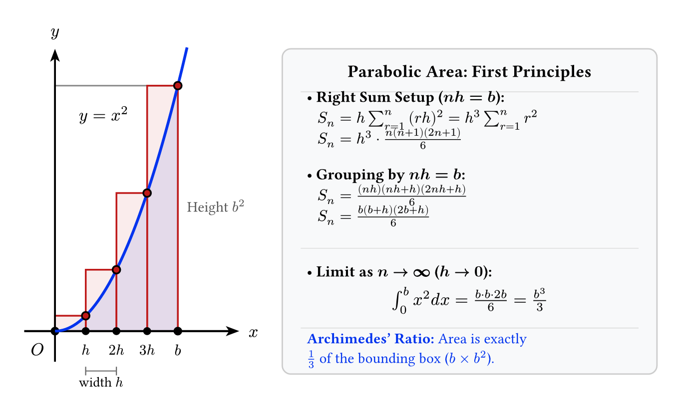
The Parabolic Area: Evaluating the Integral of Quadratic Functions

We wish to calculate the area under the standard parabola \(f(x) = x^2\) between \(x = a\) and \(x = b\):

\[\int_a^b x^2 \, dx\]

Step 1: Setting up the Right Sum

Divide \([a, b]\) into \(n\) sub-intervals of width \(h = \frac{b - a}{n}\), so \(nh = b - a\). The height of the \(r\)-th rectangle at its right endpoint is:

\[f(a + rh) = (a + rh)^2 = a^2 + 2arh + r^2 h^2\]

The total area of all \(n\) rectangles is:

\[S_n = h \sum_{r=1}^n (a + rh)^2 = h \sum_{r=1}^n \left( a^2 + 2arh + r^2 h^2 \right)\]

Step 2: Distributing the Summation

Because \(a\) and \(h\) are constant with respect to the summation index \(r\), we can pull them outside the summation signs:

\[S_n = h \left[ a^2 \sum_{r=1}^n 1 + 2ah \sum_{r=1}^n r + h^2 \sum_{r=1}^n r^2 \right]\]

Now we recall the standard finite summation formulas:

\[\sum_{r=1}^n 1 = n\]

\[\sum_{r=1}^n r = \frac{n(n + 1)}{2}\]

\[\sum_{r=1}^n r^2 = \frac{n(n + 1)(2n + 1)}{6}\]

Substituting these into our expression gives:

\[S_n = h \left[ a^2 n + 2ah \cdot \frac{n(n + 1)}{2} + h^2 \cdot \frac{n(n + 1)(2n + 1)}{6} \right]\]

Step 3: Grouping Terms by Powers of nh

Distribute the outer factor \(h\) into each term:

\[S_n = a^2 (nh) + ah^2 n(n + 1) + \frac{h^3 n(n + 1)(2n + 1)}{6}\]

To prepare for taking the limit, we combine each factor of \(h\) with a factor of \(n\):

\[h^2 n(n + 1) = (nh)(nh + h)\]

\[h^3 n(n + 1)(2n + 1) = (nh)(nh + h)(2nh + h)\]

Substituting these into \(S_n\):

\[S_n = a^2 (nh) + a (nh)(nh + h) + \frac{(nh)(nh + h)(2nh + h)}{6}\]

Step 4: Evaluating the Limit as n Approaches Infinity

Recall that \(nh = b - a\) is fixed, and as \(n \to \infty\), the strip width \(h = \frac{b - a}{n} \to 0\).

Taking the limit \(h \to 0\):

\[\lim_{h \to 0} (nh + h) = nh = b - a\]

\[\lim_{h \to 0} (2nh + h) = 2nh = 2(b - a)\]

Therefore, every term involving \(h\) vanishes:

\[\int_a^b x^2 \, dx = a^2 (b - a) + a(b - a)^2 + \frac{(b - a)(b - a)(2(b - a))}{6}\]

Simplify the third term:

\[\frac{2(b - a)^3}{6} = \frac{(b - a)^3}{3}\]

Now factor out \((b - a)\) from all three terms:

\[\int_a^b x^2 \, dx = (b - a) \left[ a^2 + a(b - a) + \frac{(b - a)^2}{3} \right]\]

Expand the expression inside the brackets:

\[a^2 + a(b - a) + \frac{(b - a)^2}{3} = a^2 + ab - a^2 + \frac{b^2 - 2ab + a^2}{3}\]

\[= ab + \frac{b^2 - 2ab + a^2}{3} = \frac{3ab + b^2 - 2ab + a^2}{3} = \frac{a^2 + ab + b^2}{3}\]

Finally, multiply by \((b - a)\):

\[\int_a^b x^2 \, dx = (b - a) \left( \frac{a^2 + ab + b^2}{3} \right) = \frac{b^3 - a^3}{3}\]

Special Case: Area from the Origin

When the lower limit is \(a = 0\), the formula simplifies to:

\[\int_0^b x^2 \, dx = \frac{b^3}{3}\]

This is the famous result first discovered by Archimedes using his geometric method of exhaustion: the area under a parabolic arch is exactly one-third of the enclosing rectangle of width \(b\) and height \(b^2\) (\(\text{Area} = \frac{1}{3} \cdot b \cdot b^2 = \frac{b^3}{3}\)).

The Exponential Area: Evaluating the Integral of Exponential Functions

Next, consider the exponential function \(f(x) = e^x\) on the interval \([a, b]\):

\[\int_a^b e^x \, dx\]

Step 1: Setting up the Right Sum

With \(h = \frac{b - a}{n}\) and \(nh = b - a\), the nodes are \(x_r = a + rh\). The Right Sum is:

\[S_n = h \sum_{r=1}^n e^{a + rh} = h \sum_{r=1}^n e^a \cdot e^{rh} = h e^a \sum_{r=1}^n (e^h)^r\]

Expanding the summation:

\[\sum_{r=1}^n (e^h)^r = e^h + e^{2h} + e^{3h} + \dots + e^{nh}\]

Step 2: Summing the Geometric Progression

This is a finite geometric progression with:

First term: \(A_1 = e^h\)
Common ratio: \(R = e^h\)
Number of terms: \(n\)

Using the sum formula for a geometric progression, \(S = A_1 \frac{R^n - 1}{R - 1}\):

\[\sum_{r=1}^n (e^h)^r = e^h \frac{(e^h)^n - 1}{e^h - 1} = e^h \frac{e^{nh} - 1}{e^h - 1}\]

Since \(nh = b - a\), the numerator becomes \(e^{b - a} - 1\). Substituting this back into the sum \(S_n\):

\[S_n = h e^a \cdot e^h \frac{e^{b - a} - 1}{e^h - 1}\]

Multiply \(e^a\) into the numerator \((e^{b - a} - 1)\):

\[e^a (e^{b - a} - 1) = e^b - e^a\]

Thus:

\[S_n = (e^b - e^a) \cdot e^h \cdot \frac{h}{e^h - 1}\]

Step 3: Evaluating the Limit using Standard Limits

Now we take the limit as \(n \to \infty\), which means \(h \to 0\).

Let us examine each factor as \(h \to 0\):

The first factor \((e^b - e^a)\) is constant.
The second factor approaches \(e^0 = 1\):

\[\lim_{h \to 0} e^h = 1\]

The third factor involves the classic standard limit for exponentials:

\[\lim_{h \to 0} \frac{e^h - 1}{h} = 1 \implies \lim_{h \to 0} \frac{h}{e^h - 1} = 1\]

Combining these limits:

\[\int_a^b e^x \, dx = \lim_{h \to 0} S_n = (e^b - e^a) \cdot 1 \cdot 1 = e^b - e^a\]

The result is remarkably clean: the area under \(y = e^x\) between \(a\) and \(b\) is simply the difference between the heights of the function at the two endpoints!

The Trigonometric Area: Evaluating the Integral of Sine

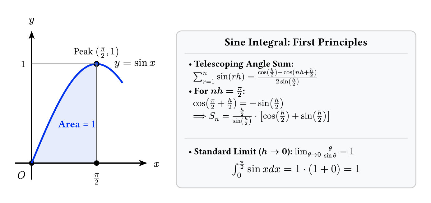
Now let us evaluate the area under the sine wave \(f(x) = \sin x\) from \(x = 0\) to \(x = \frac{\pi}{2}\):

\[\int_0^{\pi/2} \sin x \, dx\]

Step 1: Setting up the Right Sum

Here \(a = 0\) and \(b = \frac{\pi}{2}\), so the strip width is:

\[h = \frac{\pi/2 - 0}{n} = \frac{\pi}{2n} \implies nh = \frac{\pi}{2}\]

The sample points are \(x_r = 0 + rh = rh\) for \(r = 1, 2, \dots, n\). The Right Sum is:

\[S_n = h \sum_{r=1}^n \sin(rh) = h \big[ \sin(h) + \sin(2h) + \sin(3h) + \dots + \sin(nh) \big]\]

Step 2: Summing the Trigonometric Series

To sum a series of sines whose angles are in arithmetic progression, we use the standard trigonometric product-to-sum identity. Multiply and divide the entire sum by \(2 \sin\left(\frac{h}{2}\right)\):

\[2 \sin(rh) \sin\left(\frac{h}{2}\right) = \cos\left(rh - \frac{h}{2}\right) - \cos\left(rh + \frac{h}{2}\right)\]

Writing out the terms for each value of \(r\):

For \(r = 1\): \(\cos\left(\frac{h}{2}\right) - \cos\left(\frac{3h}{2}\right)\)
For \(r = 2\): \(\cos\left(\frac{3h}{2}\right) - \cos\left(\frac{5h}{2}\right)\)
For \(r = 3\): \(\cos\left(\frac{5h}{2}\right) - \cos\left(\frac{7h}{2}\right)\)
\(\dots\)
For \(r = n\): \(\cos\left(nh - \frac{h}{2}\right) - \cos\left(nh + \frac{h}{2}\right)\)

Adding all these equations, intermediate terms cancel out telescopically! Only the very first term and the very last term survive:

\[\sum_{r=1}^n 2 \sin(rh) \sin\left(\frac{h}{2}\right) = \cos\left(\frac{h}{2}\right) - \cos\left(nh + \frac{h}{2}\right)\]

Dividing by \(2 \sin\left(\frac{h}{2}\right)\):

\[\sum_{r=1}^n \sin(rh) = \frac{\cos\left(\frac{h}{2}\right) - \cos\left(nh + \frac{h}{2}\right)}{2 \sin\left(\frac{h}{2}\right)}\]

Step 3: Substituting nh and Simplifying

Recall that \(nh = \frac{\pi}{2}\). Therefore:

\[\cos\left(nh + \frac{h}{2}\right) = \cos\left(\frac{\pi}{2} + \frac{h}{2}\right) = - \sin\left(\frac{h}{2}\right)\]

Substituting this into the numerator:

\[\cos\left(\frac{h}{2}\right) - \left(-\sin\left(\frac{h}{2}\right)\right) = \cos\left(\frac{h}{2}\right) + \sin\left(\frac{h}{2}\right)\]

So the sum becomes:

\[\sum_{r=1}^n \sin(rh) = \frac{\cos\left(\frac{h}{2}\right) + \sin\left(\frac{h}{2}\right)}{2 \sin\left(\frac{h}{2}\right)}\]

Now multiply by the outer factor \(h\) to get \(S_n\):

\[S_n = h \cdot \frac{\cos\left(\frac{h}{2}\right) + \sin\left(\frac{h}{2}\right)}{2 \sin\left(\frac{h}{2}\right)} = \frac{h/2}{\sin(h/2)} \cdot \left[ \cos\left(\frac{h}{2}\right) + \sin\left(\frac{h}{2}\right) \right]\]

Step 4: Evaluating the Limit using Standard Trigonometric Limits

As \(n \to \infty\), \(h \to 0\), and therefore \(\frac{h}{2} \to 0\).

From our study of standard limits:

\[\lim_{\theta \to 0} \frac{\sin \theta}{\theta} = 1 \implies \lim_{h \to 0} \frac{h/2}{\sin(h/2)} = 1\]

Furthermore:

\[\lim_{h \to 0} \cos\left(\frac{h}{2}\right) = \cos(0) = 1\]

\[\lim_{h \to 0} \sin\left(\frac{h}{2}\right) = \sin(0) = 0\]

Putting these limits together:

\[\int_0^{\pi/2} \sin x \, dx = \lim_{h \to 0} S_n = 1 \cdot (1 + 0) = 1\]

The exact area under a quarter-period of the sine wave is precisely \(1\).

The Limitation of First-Principles Summation

While the three calculations above are elegant, consider what was required:

For \(x^2\), we needed the formula for the sum of squares \(\sum r^2\). For \(x^3\), we would need \(\sum r^3\), and for \(x^k\), higher Faulhaber formulas.
For \(e^x\), we relied on the formula for a geometric progression.
For \(\sin x\), we relied on a specialized telescoping trigonometric identity.

What happens if we try to evaluate an integral as simple as:

\[\int_0^1 \frac{1}{1 + x^2} \, dx \quad \text{or} \quad \int_1^2 \frac{1}{x} \, dx \quad \text{or} \quad \int_0^1 \sqrt{1 - x^2} \, dx\]

Setting up the Riemann sum for \(\frac{1}{1 + x^2}\) requires evaluating:

\[\sum_{r=1}^n \frac{1}{1 + (r/n)^2} = \sum_{r=1}^n \frac{n^2}{n^2 + r^2}\]

There is no elementary algebraic formula to sum \(\frac{1}{n^2 + r^2}\) in finite terms!

Evaluating integrals purely by calculating limits of rectangular sums is a dead end for general functions. We need general laws and properties that allow us to manipulate and compute integrals without summing rectangles every time.

Fundamental Properties of Definite Integrals

By viewing the definite integral as the accumulated area under a curve, we can understand its fundamental operational properties intuitively.

Property 1: Integration Over a Single Point

\[\int_a^a f(x) \, dx = 0\]

Geometric Meaning:

The interval of integration has length:

\[\text{Width} = a - a = 0\]

A vertical line segment has height \(f(a)\) but zero width. Since \(\text{Area} = \text{width} \times \text{height} = 0 \times f(a) = 0\), a region of zero width encloses zero area.

Property 2: Reversal of Limits

\[\int_a^b f(x) \, dx = - \int_b^a f(x) \, dx\]

Geometric and Algebraic Meaning:

When integrating from \(a\) to \(b\), the width of each strip is:

\[\Delta x = \frac{b - a}{n}\]

If we integrate in the reverse direction, from \(b\) back to \(a\), the displacement of each step is:

\[\Delta x_{\text{rev}} = \frac{a - b}{n} = - \left( \frac{b - a}{n} \right) = - \Delta x\]

Because every strip width acquires a minus sign, the entire sum is negated:

\[\sum f(x_r) \, \Delta x_{\text{rev}} = - \sum f(x_r) \, \Delta x\]

This property ensures that the algebra of integration behaves consistently regardless of which direction we traverse an interval.

Property 3: The Dummy Variable Property

\[\int_a^b f(x) \, dx = \int_a^b f(t) \, dt = \int_a^b f(u) \, du\]

Geometric Meaning:

A definite integral evaluates to a single fixed numerical value—the geometric area of the region bounded by \(y = f(x)\), the horizontal axis, and the vertical lines at the limits.

The letter \(x\) is merely a label for the horizontal axis. If we rename the horizontal axis from \(x\) to \(t\) or \(u\), the curve \(y = f(t)\) and the boundary lines \(t = a\) and \(t = b\) define the exact same physical region with the exact same area. The variable of integration is called a dummy variable because it does not appear in the final answer.

Property 4: Constant Multiple Property

For any constant \(k\):

\[\int_a^b k f(x) \, dx = k \int_a^b f(x) \, dx\]

Geometric Meaning:

Multiplying a function by a constant factor \(k\) stretches (if \(k > 1\)) or compresses (if \(0 < k < 1\)) the height of every point on the curve by \(k\).

In our rectangular approximation, the height of every strip changes from \(f(x_r)\) to \(k f(x_r)\). Therefore, the area of every strip is multiplied by \(k\):

\[\text{Area}_r = h \cdot \big( k f(x_r) \big) = k \cdot \big( h f(x_r) \big)\]

Factoring \(k\) out of the entire sum:

\[\sum_{r=1}^n k f(x_r) h = k \sum_{r=1}^n f(x_r) h\]

Taking the limit as \(n \to \infty\) confirms that the total area scales by the factor \(k\).

Property 5: Sum and Difference Property

\[\int_a^b \big[ f(x) \pm g(x) \big] \, dx = \int_a^b f(x) \, dx \pm \int_a^b g(x) \, dx\]

Geometric Meaning:

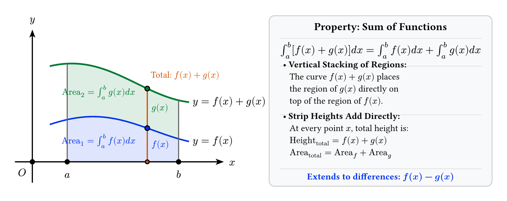
Consider two positive functions \(f(x)\) and \(g(x)\). The combined function \(f(x) + g(x)\) represents the total height obtained by stacking the region under \(g(x)\) directly on top of the region under \(f(x)\).

At each strip, the combined height is:

\[\text{Height}_r = f(x_r) + g(x_r)\]

The area of the \(r\)-th rectangular strip is:

\[h \big[ f(x_r) + g(x_r) \big] = h f(x_r) + h g(x_r)\]

Summing across all \(n\) strips:

\[\sum_{r=1}^n h \big[ f(x_r) + g(x_r) \big] = \sum_{r=1}^n h f(x_r) + \sum_{r=1}^n h g(x_r)\]

Taking the limit as \(n \to \infty\), the total area under the combined curve equals the sum of the areas of the two individual regions. The same logic applies to differences \(f(x) - g(x)\) by subtracting heights.

Property 6: Splitting the Interval of Integration

For any three points \(a\), \(b\), and \(c\):

\[\int_a^b f(x) \, dx = \int_a^c f(x) \, dx + \int_c^b f(x) \, dx\]

Geometric Meaning:

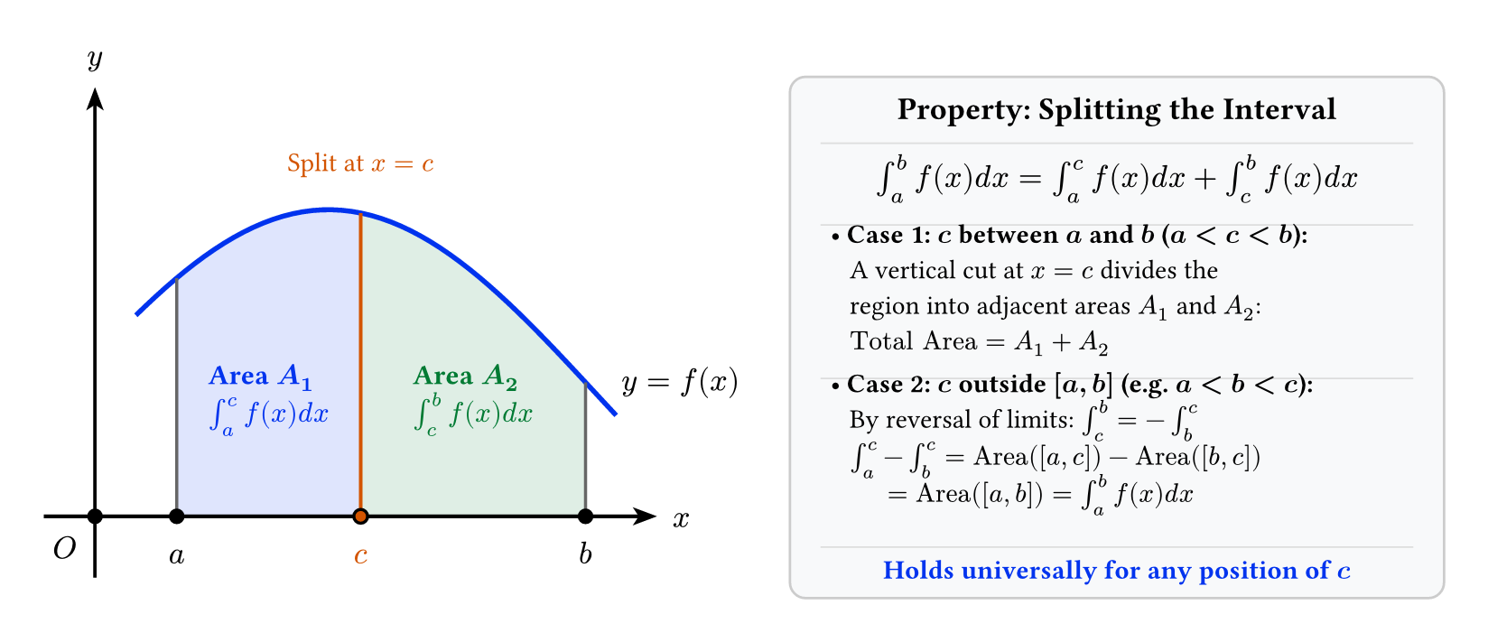
Case 1: When c lies between a and b (\(a < c < b\))

Imagine erecting a vertical barrier at \(x = c\). This barrier divides the total region under \(y = f(x)\) from \(a\) to \(b\) into two separate, adjacent sub-regions:

A left sub-region extending from \(x = a\) to \(x = c\), with area \(\int_a^c f(x) \, dx\).
A right sub-region extending from \(x = c\) to \(x = b\), with area \(\int_c^b f(x) \, dx\).

Because the two sub-regions meet along the line \(x = c\) (which has zero width and encloses no area of its own), the total area is simply the sum of the two component areas:

\[\text{Total Area} = \text{Area}_1 + \text{Area}_2\]

\[\int_a^b f(x) \, dx = \int_a^c f(x) \, dx + \int_c^b f(x) \, dx\]

Case 2: When c lies outside \([a, b]\)

Remarkably, this identity holds even when \(c\) lies completely outside the interval \([a, b]\)!

Suppose, for example, that \(c > b\), so the order of points is \(a < b < c\).

From Case 1, since \(b\) lies between \(a\) and \(c\):

\[\int_a^c f(x) \, dx = \int_a^b f(x) \, dx + \int_b^c f(x) \, dx\]

Subtracting \(\int_b^c f(x) \, dx\) from both sides:

\[\int_a^b f(x) \, dx = \int_a^c f(x) \, dx - \int_b^c f(x) \, dx\]

Now apply Property 2 (reversal of limits) to the second integral: \(-\int_b^c f(x) \, dx = +\int_c^b f(x) \, dx\). Substituting this in:

\[\int_a^b f(x) \, dx = \int_a^c f(x) \, dx + \int_c^b f(x) \, dx\]

The equation holds universally. Interval splitting behaves like vector displacement along the \(x\)-axis: moving from \(a\) to \(c\) and then from \(c\) to \(b\) produces a net displacement from \(a\) to \(b\), regardless of where the waypoint \(c\) is situated.

Summary of Core Properties

Property	Formula	Geometric Interpretation
Zero Width	\(\int_a^a f(x) \, dx = 0\)	A strip of zero width encloses zero area.
Reversal of Limits	\(\int_a^b f(x) \, dx = - \int_b^a f(x) \, dx\)	Reversing traversal direction negates strip widths \(\Delta x\).
Dummy Variable	\(\int_a^b f(x) \, dx = \int_a^b f(t) \, dt\)	The area is a fixed number; axis label does not affect area.
Constant Multiple	\(\int_a^b k f(x) \, dx = k \int_a^b f(x) \, dx\)	Scaling all heights by \(k\) scales the total area by \(k\).
Sum / Difference	\(\int_a^b [f(x) \pm g(x)] \, dx = \int_a^b f(x) \, dx \pm \int_a^b g(x) \, dx\)	Stacking or subtracting heights adds or subtracts areas.
Interval Splitting	\(\int_a^b f(x) \, dx = \int_a^c f(x) \, dx + \int_c^b f(x) \, dx\)	Dividing an area with a vertical line at \(x = c\).