Introduction to Definite Integration

In Chapter 23, we studied indefinite integration as the reverse process of differentiation: given a derivative \(f(x)\), we sought a primitive function \(F(x)\) such that \(F'(x) = f(x)\).

We now turn to a foundational geometric problem that occupied mathematicians from ancient Greece to the seventeenth century:

How can we compute the exact area of a plane region bounded by curved boundaries?

In elementary geometry, finding the area of a polygon is straightforward because any straight-edged figure can be split into a finite number of triangles. But the moment a boundary curves continuously, ordinary geometry cannot give us an exact answer.

To solve this, Archimedes introduced the method of exhaustion, approximating curved shapes with straight-sided polygons. In the seventeenth and nineteenth centuries, Newton, Leibniz, Cauchy, and Riemann transformed this geometric idea into the modern theory of definite integration—a systematic method of slicing a curved region into vanishingly thin rectangular strips and taking the limit of their sum.

The Curvilinear Trapezoid

To analyze curved areas mathematically, we set up the problem using Cartesian coordinates.

Let \(f(x)\) be a continuous, positive function on a closed interval \([a, b]\), where \(a < b\):

\[f(x) \ge 0 \quad \text{for all } x \in [a, b]\]

Consider the region bounded by four boundaries:

The continuous curve \(y = f(x)\) along the top.
The \(x\)-axis (\(y = 0\)) along the bottom.
The vertical line \(x = a\) on the left.
The vertical line \(x = b\) on the right.

This region is called a curvilinear trapezoid.

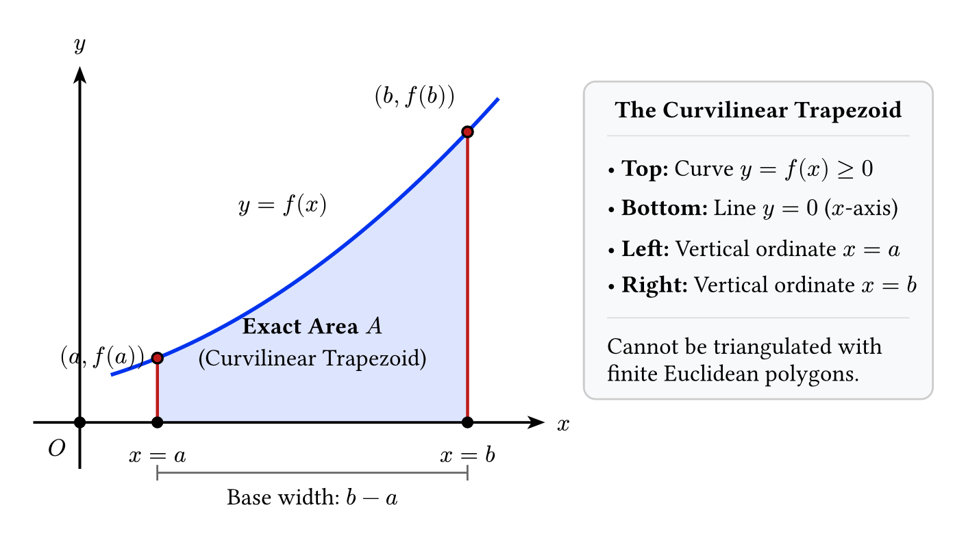
If the upper boundary were a straight line, this would be an ordinary trapezoid with area \((b - a) \cdot \frac{f(a) + f(b)}{2}\). But because \(y = f(x)\) bends and curves, simple geometry formulas cannot give its exact area. Our goal is to find the exact area \(A\) of this region.

The Slicing Strategy: Partitioning the Interval

To find the area of an unfamiliar curved shape, the most natural strategy is to approximate it using the simplest shape whose area we know: the rectangle.

Let us divide the base interval \([a, b]\) into \(n\) equal sub-intervals.

Step Width

Since the total distance from \(a\) to \(b\) has length \(b - a\), each of the \(n\) sub-intervals has an equal width \(h\):

\[h = \frac{b - a}{n}\]

Multiplying both sides by \(n\) gives the fundamental relation:

\[nh = b - a \iff b = a + nh\]

The Division Points

We denote the \(n + 1\) division points by \(x_0, x_1, x_2, \dots, x_n\), where:

\[x_0 = a\]

\[x_1 = a + h\]

\[x_2 = a + 2h\]

\[\vdots\]

\[x_r = a + rh\]

\[\vdots\]

\[x_n = a + nh = b\]

In general, the \(r\)-th division point is:

\[x_r = a + rh \quad \text{for } r = 0, 1, 2, \dots, n\]

These points divide \([a, b]\) into \(n\) consecutive sub-intervals:

\[[x_0, x_1] = [a, a + h], \quad [x_1, x_2] = [a + h, a + 2h], \quad \dots, \quad [x_{r-1}, x_r] = [a + (r-1)h, a + rh]\]

Each sub-interval has the exact same width:

\[x_r - x_{r-1} = h\]

Two Natural Approximations: Left Sum and Right Sum

To see how rectangular approximations work, let us first consider a function \(f(x)\) that is strictly increasing on \([a, b]\):

\[x_1 < x_2 \implies f(x_1) < f(x_2)\]

On any sub-interval \([x_{r-1}, x_r]\), the function climbs steadily from its lowest value at the left endpoint to its highest value at the right endpoint:

\[f(x_{r-1}) \le f(x) \le f(x_r)\]

This allows us to construct two different rectangular approximations on each strip: one that sits beneath the curve, and one that stands above it.

The Left Sum (Inscribed Rectangles)

On each sub-interval \([x_{r-1}, x_r]\), build a rectangle of base \(h\) with height chosen at the left endpoint:

\[\text{Height} = f(x_{r-1}) = f(a + (r-1)h)\]

Because \(f(x)\) is increasing, this rectangle lies entirely beneath the curve. It is an inscribed rectangle.

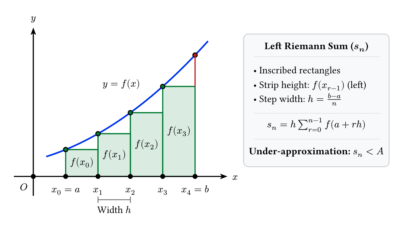
The area of the \(r\)-th inscribed rectangle is:

\[\text{Area} = \text{base} \times \text{height} = h \cdot f(a + (r-1)h)\]

Adding up the areas of all \(n\) inscribed rectangles gives the Left Sum, denoted by \(s_n\):

\[s_n = h \Big[ f(a) + f(a + h) + f(a + 2h) + \dots + f(a + (n-1)h) \Big]\]

Using sigma notation, with index \(r\) running from \(0\) to \(n-1\):

\[s_n = h \sum_{r=0}^{n-1} f(a + rh)\]

Because every inscribed rectangle lies completely inside the curvilinear trapezoid, their total area is an underestimate of the true area \(A\):

\[s_n < A\]

The Right Sum (Circumscribed Rectangles)

Next, on each sub-interval \([x_{r-1}, x_r]\), build a rectangle of base \(h\) with height chosen at the right endpoint:

\[\text{Height} = f(x_r) = f(a + rh)\]

Because \(f(x)\) is increasing, the top of this rectangle juts out above the curve. It is a circumscribed rectangle.

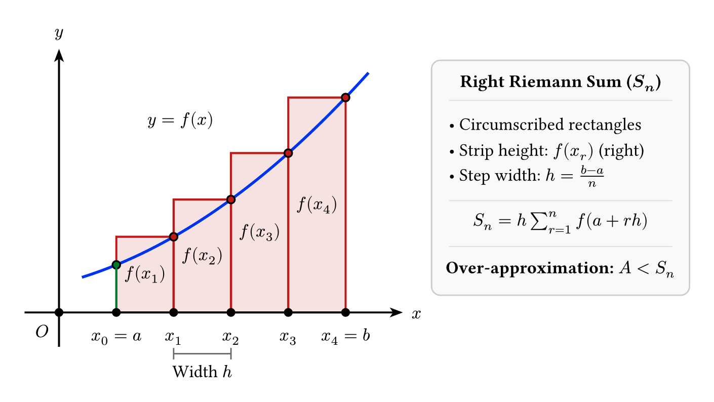
The area of the \(r\)-th circumscribed rectangle is:

\[\text{Area} = \text{base} \times \text{height} = h \cdot f(a + rh)\]

Adding up the areas of all \(n\) circumscribed rectangles gives the Right Sum, denoted by \(S_n\):

\[S_n = h \Big[ f(a + h) + f(a + 2h) + f(a + 3h) + \dots + f(a + nh) \Big]\]

Using sigma notation, with index \(r\) running from \(1\) to \(n\):

\[S_n = h \sum_{r=1}^{n} f(a + rh)\]

Because every circumscribed rectangle extends above the curve, their total area is an overestimate of the true area \(A\):

\[A < S_n\]

Trapping the Exact Area

Putting both inequalities together, the true area \(A\) of the curvilinear trapezoid is strictly trapped between the inscribed rectangles (Left Sum) and the circumscribed rectangles (Right Sum):

\[s_n < A < S_n\]

Written out with summation formulas:

\[h \sum_{r=0}^{n-1} f(a + rh) < A < h \sum_{r=1}^{n} f(a + rh)\]

No matter how many slices \(n\) we choose, the true area \(A\) is always trapped between these two easy-to-calculate rectangular sums.

The Vanishing Error and Telescoping Cancellation

How close are our two estimates \(s_n\) and \(S_n\) to each other? Let us find their difference:

\[S_n - s_n = h \sum_{r=1}^n f(a + rh) - h \sum_{r=0}^{n-1} f(a + rh)\]

Writing out both sums side by side reveals a simple and beautiful cancellation:

\[S_n = h \Big[ f(a+h) + f(a+2h) + \dots + f(a+(n-1)h) + f(a+nh) \Big]\]

\[s_n = h \Big[ f(a) + f(a+h) + f(a+2h) + \dots + f(a+(n-1)h) \Big]\]

Every intermediate term from \(f(a+h)\) through \(f(a+(n-1)h)\) cancels out completely! Only the first and last terms survive:

\[S_n - s_n = h \Big[ f(a + nh) - f(a) \Big]\]

Since \(a + nh = b\) and \(h = \frac{b - a}{n}\), this simplifies to:

\[S_n - s_n = \frac{b - a}{n} \Big[ f(b) - f(a) \Big]\]

Notice how powerful this result is:

The numbers \(a\), \(b\), \(f(a)\), and \(f(b)\) are fixed constants that do not change with \(n\).
Therefore, the bracket \((b - a)[f(b) - f(a)]\) is just a fixed number.
As we increase the number of slices \(n\) toward infinity (\(n \to \infty\)), the fraction \(\frac{1}{n} \to 0\).

Taking the limit as \(n \to \infty\):

\[\lim_{n \to \infty} (S_n - s_n) = \lim_{n \to \infty} \left( \frac{b - a}{n} \big[ f(b) - f(a) \big] \right) = 0\]

The difference between the circumscribed overestimate \(S_n\) and the inscribed underestimate \(s_n\) shrinks to zero!

The Squeeze Principle: Finding the Exact Area

Because the true area \(A\) is permanently trapped between the two sums:

\[s_n < A < S_n\]

and the gap between them vanishes as \(n \to \infty\):

\[\lim_{n \to \infty} (S_n - s_n) = 0\]

by the Sandwich (Squeeze) Theorem, both sequences are forced to converge to the exact same value. That common value must be the true area \(A\):

\[A = \lim_{n \to \infty} s_n = \lim_{n \to \infty} S_n\]

Visualizing the Convergence: Coarse vs. Fine Partitions

To see why the error disappears, look at what happens when we increase the number of slices from a coarse partition (\(n = 4\)) to a finer partition (\(n = 16\)).

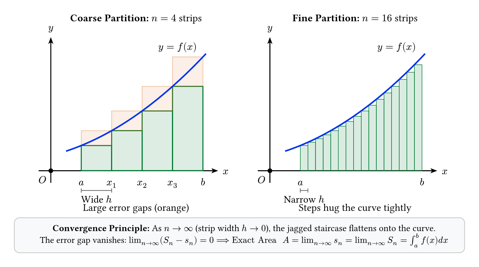
With \(n = 4\), the wide rectangular steps create large, visible gaps between the rectangles and the curve.

When we refine the partition to \(n = 16\), the step width \(h\) is cut to one-fourth of its original size. The jagged staircase flattens against the smooth curve, and the gap between the upper and lower sums practically disappears. In the limit as \(n \to \infty\) (\(h \to 0\)), the stepped boundary becomes indistinguishable from the curve itself.

Definition of the Definite Integral

Because both the Left Sum and the Right Sum converge to the exact area \(A\), we can write \(A\) as either limit:

\[A = \lim_{n \to \infty} h \sum_{r=0}^{n-1} f(a + rh) = \lim_{n \to \infty} h \sum_{r=1}^{n} f(a + rh)\]

where \(h = \frac{b - a}{n}\) and \(nh = b - a\).

This fundamental limit is called the Definite Integral of \(f(x)\) from \(a\) to \(b\), and is written as:

\[\int_a^b f(x) \, dx\]

Thus:

\[\int_a^b f(x) \, dx = \lim_{n \to \infty} \frac{b - a}{n} \sum_{r=1}^n f\left(a + r \frac{b - a}{n}\right) = \lim_{h \to 0} h \sum_{r=1}^n f(a + rh)\]

Anatomy of the Integral Symbol

Leibniz introduced this notation to represent the limiting sum from which the definite integral arises:

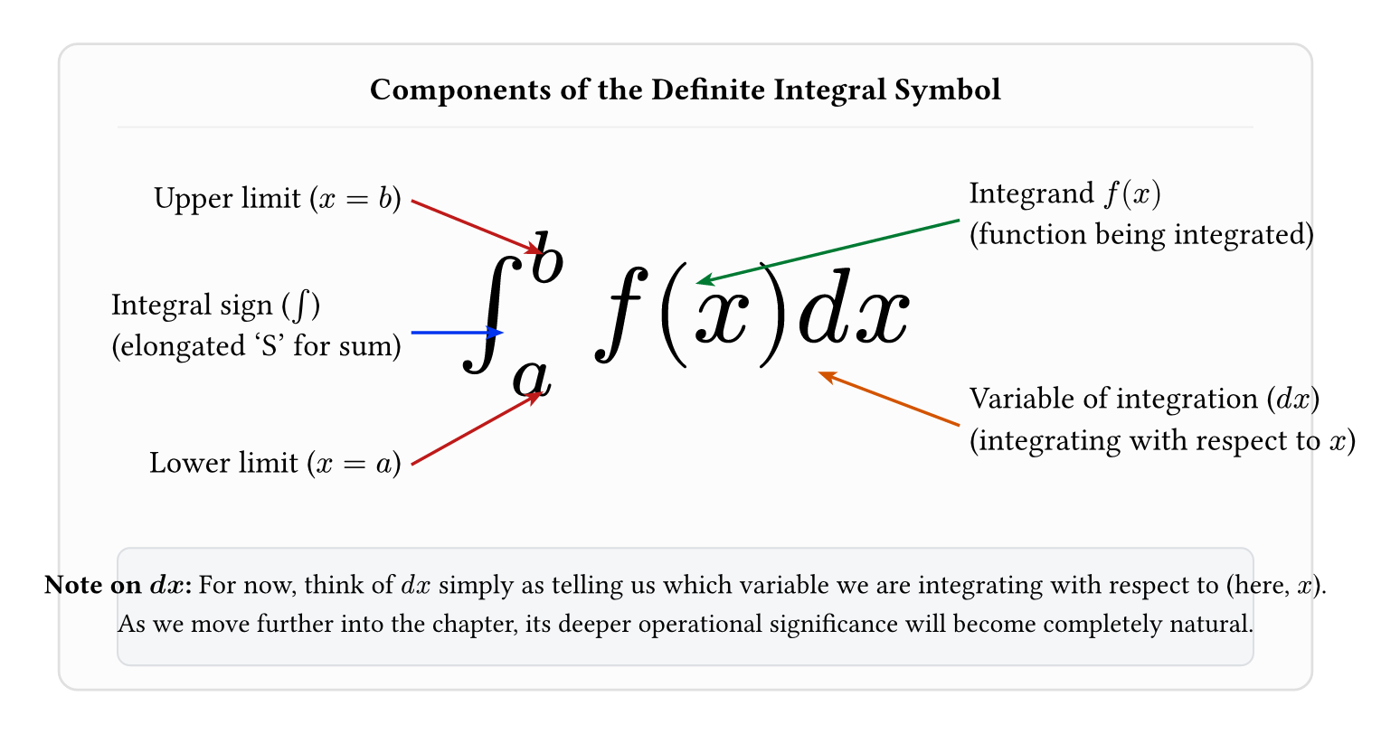
The Integral Sign (\(\int\)): An elongated letter "S" (from the Latin Summa, meaning sum). It represents the continuous limit of the summation symbol \(\sum\).
The Limits of Integration (\(a\) and \(b\)): The interval \([a, b]\) along the \(x\)-axis over which the accumulation occurs. The number \(a\) is the lower limit, and \(b\) is the upper limit.
The Integrand (\(f(x)\)): The function being integrated, which specifies the height of the curve at each point.
The Variable of Integration (\(dx\)): Specifies the active variable with respect to which the integration is performed (here, \(x\)).

Note on \(dx\): At this introductory stage, do not worry about treating \(dx\) as an "infinitesimal quantity." For now, it simply tells us which variable we are integrating with respect to. As we advance through subsequent sections—especially when we study integration by substitution and the Fundamental Theorem of Calculus—its deeper algebraic and geometric role will become completely clear.

Extending Beyond Strictly Increasing Functions

Our initial derivation assumed that \(f(x)\) is strictly positive and strictly increasing on \([a, b]\). While this made the geometry easy to visualize, the definite integral works for all continuous functions.

Let us examine what occurs when these conditions are relaxed.

Strictly Decreasing Positive Functions

Suppose \(f(x) \ge 0\) is continuous and strictly decreasing on \([a, b]\):

\[x_1 < x_2 \implies f(x_1) > f(x_2)\]

On any sub-interval \([x_{r-1}, x_r]\), the function drops as we move from left to right. Therefore, the roles of the endpoints reverse:

The maximum height on the strip occurs at the left endpoint: \(f(x_{r-1})\).
The minimum height on the strip occurs at the right endpoint: \(f(x_r)\).

Because of this reversal:

1. Left Sum (Circumscribed Rectangles):

The Left Sum evaluates heights at left endpoints, which are now the highest points on each strip. Hence, the rectangles extend above the curve, making the Left Sum an overestimate:

\[s_n^{\text{left}} = h \sum_{r=0}^{n-1} f(a + rh) > A\]

2. Right Sum (Inscribed Rectangles):

The Right Sum evaluates heights at right endpoints, which are now the lowest points on each strip. Hence, the rectangles sit beneath the curve, making the Right Sum an underestimate:

\[S_n^{\text{right}} = h \sum_{r=1}^{n} f(a + rh) < A\]

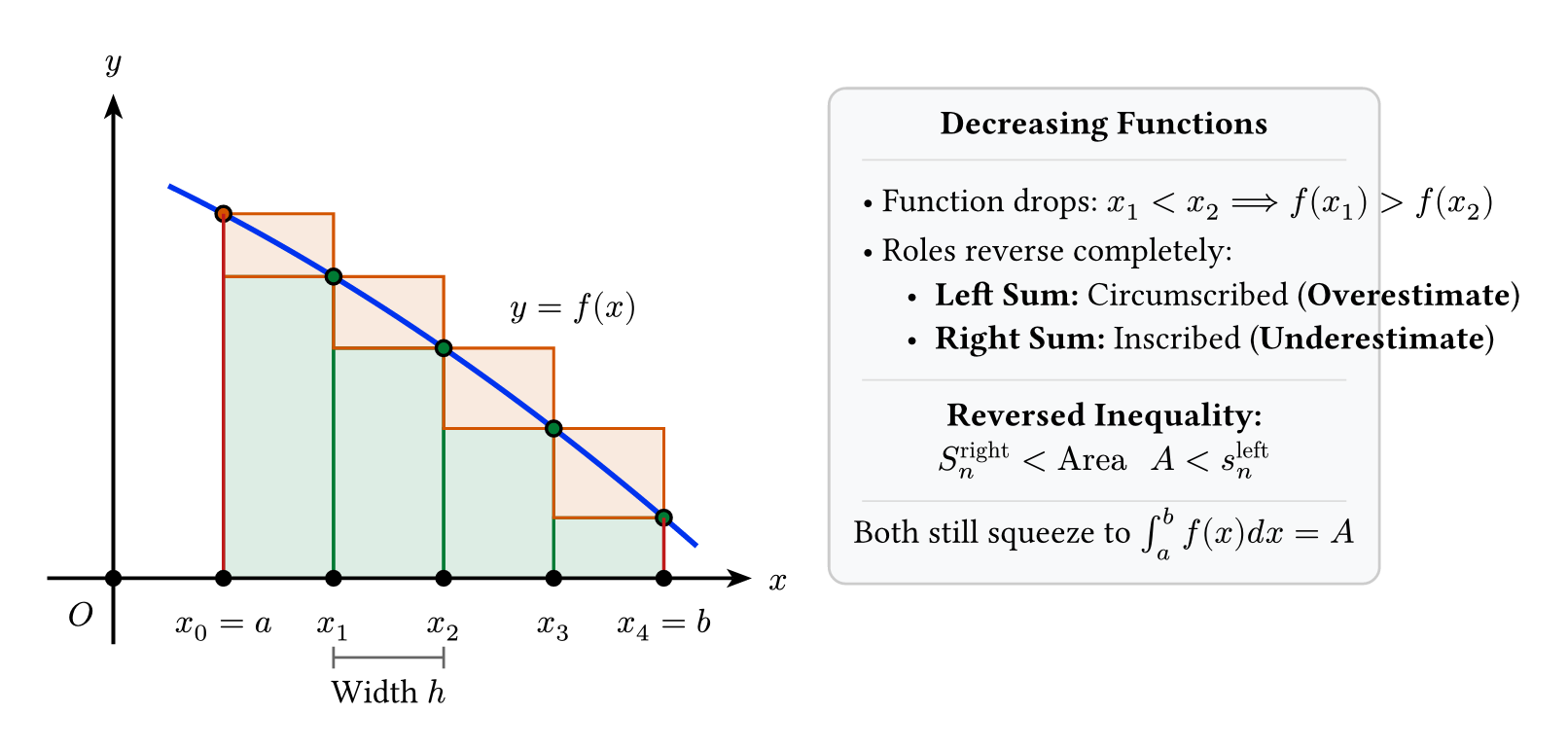
The bounding inequality simply reverses:

\[S_n^{\text{right}} < A < s_n^{\text{left}}\]

The difference between the two sums still collapses telescopically:

\[s_n^{\text{left}} - S_n^{\text{right}} = h \big[ f(a) - f(b) \big] = \frac{b - a}{n} \big[ f(a) - f(b) \big]\]

As \(n \to \infty\), this difference approaches zero:

\[\lim_{n \to \infty} \left( s_n^{\text{left}} - S_n^{\text{right}} \right) = 0\]

By the Sandwich Theorem, both sums squeeze down to the exact same limit, which is once again the exact area \(A = \int_a^b f(x) \, dx\).

Functions with Both Increasing and Decreasing Regions

What if a positive function \(f(x) \ge 0\) rises on some intervals and falls on others (for example, a wave or a curve with peaks and valleys)?

On intervals where the curve climbs, the left endpoint gives an inscribed rectangle (underestimate) and the right endpoint gives a circumscribed rectangle (overestimate). On intervals where the curve descends, the roles reverse. On intervals containing local peaks or troughs, neither endpoint represents the extreme value of the strip.

Consequently, we cannot say that the Left Sum is always an underestimate or that the Right Sum is always an overestimate. On some strips the rectangle overshoots the curve, while on others it falls short.

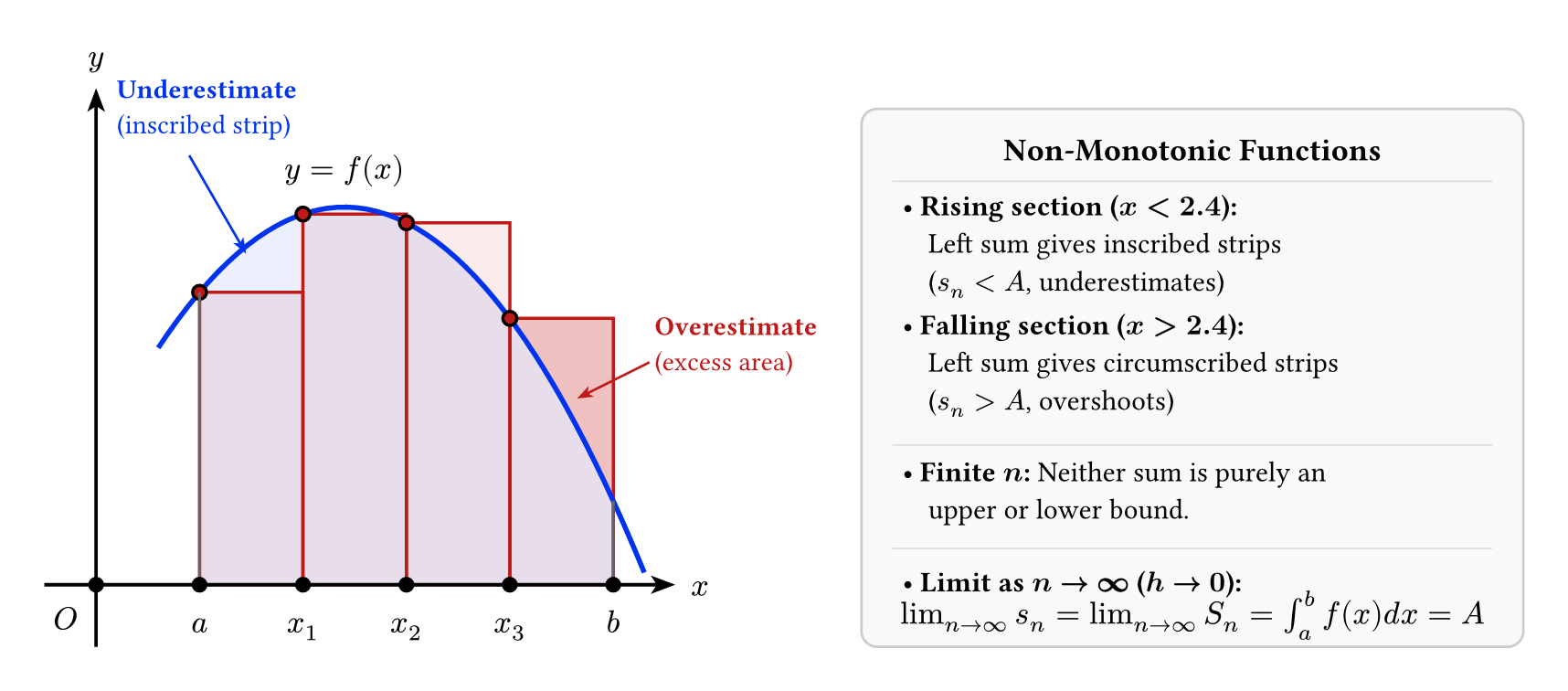
However, as we divide \([a, b]\) into increasingly fine strips (\(n \to \infty\), \(h \to 0\)), the width \(h\) of every sub-interval shrinks toward zero. Because \(f(x)\) is continuous, the difference between the highest value and lowest value of the function on each tiny strip vanishes.

Whether we evaluate the height of each rectangle at the left endpoint, the right endpoint, the midpoint, or any point on the strip, the sum converges to the exact same unique number:

\[\int_a^b f(x) \, dx = \text{Area } A\]

Negative Functions: When the Curve Lies Below the Axis

Now consider what happens if the function is strictly negative on \([a, b]\):

\[f(x) \le 0 \quad \text{for all } x \in [a, b]\]

In this case, the entire curve \(y = f(x)\) lies beneath the \(x\)-axis.

If we build our rectangular sum using the definition of the definite integral:

\[S_n = h \sum_{r=1}^n f(a + rh)\]

let us look at the sign of each term:

The width of each strip \(h = \frac{b - a}{n}\) is positive (\(h > 0\)).
But the function values are all negative (\(f(a + rh) \le 0\)).

Because we are multiplying a positive width by a negative value, every term in the sum is negative! Consequently, the sum \(S_n\) is negative, and taking the limit gives a negative number:

\[\int_a^b f(x) \, dx = \lim_{n \to \infty} h \sum_{r=1}^n f(a + rh) \le 0\]

This immediately raises a natural question: How can an area be negative? In geometry, area can never be negative—a room cannot have an area of \(-20\text{ m}^2\).

To understand what the integral represents here, let us look at the true geometric height of each strip:

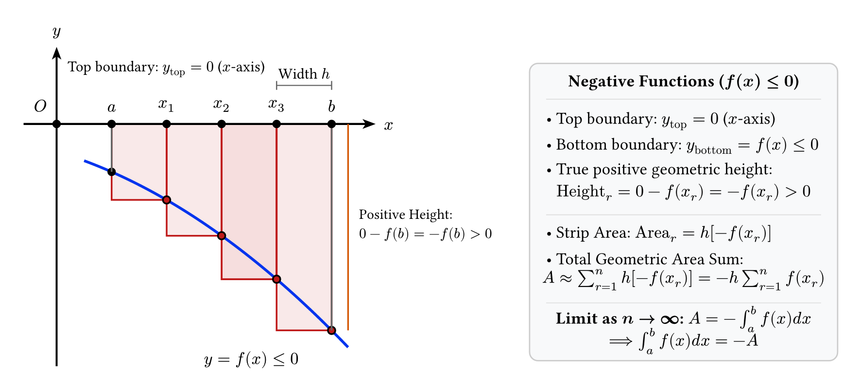
1. Finding the Positive Geometric Height:

In coordinate geometry, the height (distance) of any vertical strip is the upper boundary minus the lower boundary:

\[\text{Height}_r = y_{\text{top}} - y_{\text{bottom}} = 0 - f(a + rh) = -f(a + rh)\]

Because \(f(a + rh)\) is negative, the quantity \(-f(a + rh)\) is a strictly positive number.

2. Writing the Geometric Area as a Sum:

The actual geometric area of the \(r\)-th rectangular strip is:

\[\text{Area}_r = \text{base} \times \text{height} = h \cdot \big(-f(a + rh)\big)\]

Adding up the areas of all \(n\) rectangles gives the approximation for the true geometric area \(A\):

\[A \approx \sum_{r=1}^n h \cdot \big(-f(a + rh)\big)\]

3. Factoring Out the Negative Sign:

We can factor out the minus sign from every term in the summation:

\[A \approx - h \sum_{r=1}^n f(a + rh) = - S_n\]

4. Taking the Limit:

Now take the limit as \(n \to \infty\) (\(h \to 0\)):

\[A = \lim_{n \to \infty} \left[ - h \sum_{r=1}^n f(a + rh) \right] = - \lim_{n \to \infty} h \sum_{r=1}^n f(a + rh)\]

Recognizing the limit on the right as the definite integral \(\int_a^b f(x) \, dx\):

\[A = - \int_a^b f(x) \, dx\]

Multiplying both sides by \(-1\) reveals the key relationship:

\[\int_a^b f(x) \, dx = - A\]

This resolves the puzzle completely through summation formulas:

The definite integral does not force heights to be positive. Because it multiplies the width \(h\) by the raw function value \(f(x)\), any region below the \(x\)-axis produces a negative sum. Hence, for a curve below the \(x\)-axis, the definite integral evaluates to the negative of the true geometric area.

The Definite Integral as Net Signed Area

What happens if a function takes both positive and negative values on \([a, b]\), crossing the \(x\)-axis at one or more points?

Consider a continuous function \(f(x)\) that is positive on \([a, c]\) and negative on \([c, b]\), crossing the \(x\)-axis at \(x = c\).

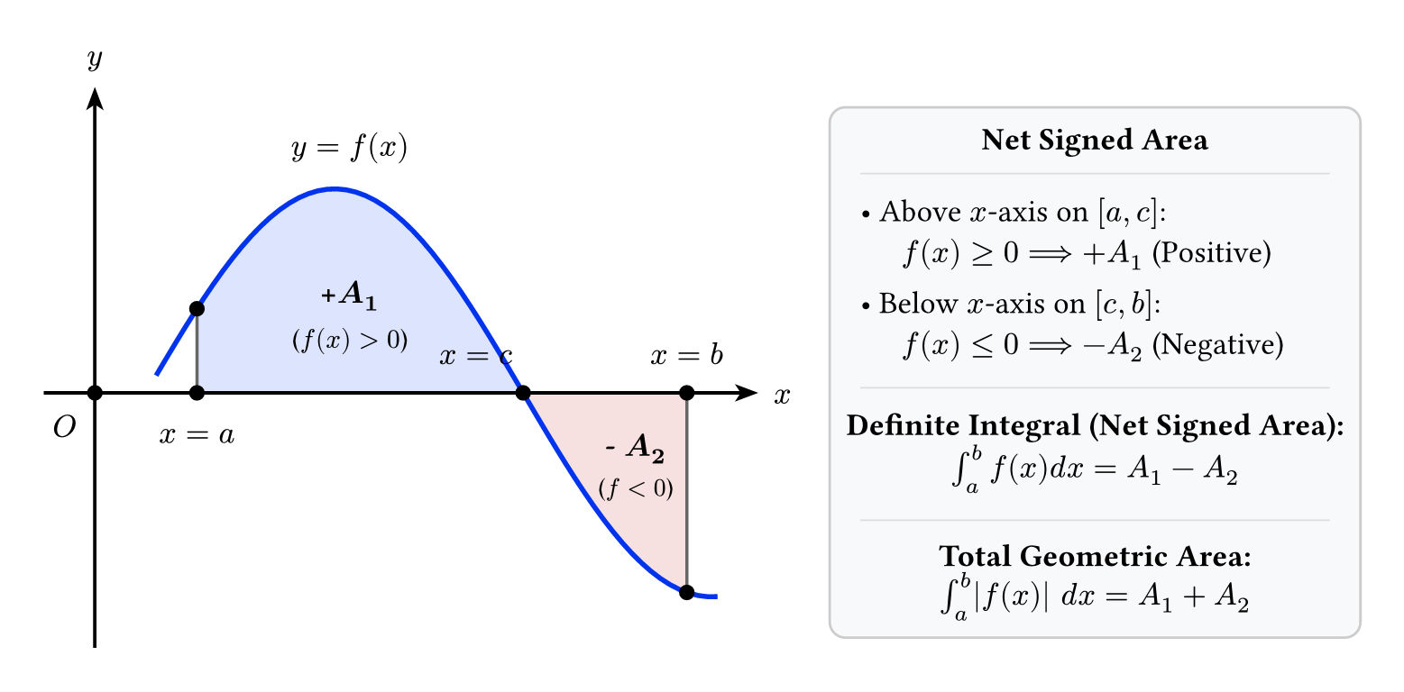
The region bounded between the curve and the \(x\)-axis is split into two distinct parts:

A lobe above the \(x\)-axis on \([a, c]\), with geometric area \(A_1 > 0\).
A lobe below the \(x\)-axis on \([c, b]\), with geometric area \(A_2 > 0\).

Because the definite integral accumulates positive values where \(f(x) > 0\) and negative values where \(f(x) < 0\), it calculates the Net Signed Area:

\[\int_a^b f(x) \, dx = A_1 - A_2\]

This distinction is crucial for Class 11 and 12 students:

Net Signed Area (The Definite Integral):

Regions above the \(x\)-axis are counted as positive (\(+A_1\)), while regions below the \(x\)-axis are counted as negative (\(-A_2\)). If both lobes are identical in size (\(A_1 = A_2\)), the definite integral is precisely zero:

\[\int_a^b f(x) \, dx = 0\]

even though a substantial geometric region is enclosed between the curve and the axis!

Total Geometric Area:

If a problem asks for the physical, non-negative area enclosed between the curve and the \(x\)-axis, we must take the absolute value of the function \(|f(x)|\), or split the integral at the crossing points:

\[\text{Total Geometric Area} = \int_a^b |f(x)| \, dx = \int_a^c f(x) \, dx + \int_c^b \big(-f(x)\big) \, dx = A_1 + A_2\]

Summary

Slicing and Partitioning

To compute the area under a curve, divide \([a, b]\) into \(n\) equal strips of width \(h = \frac{b - a}{n}\), with division points \(x_r = a + rh\) for \(r = 0, 1, \dots, n\).

Trapping the Area (Monotonic Functions)

For a strictly increasing function, the Left Sum forms inscribed rectangles (underestimate) and the Right Sum forms circumscribed rectangles (overestimate):

\[s_n^{\text{left}} < A < S_n^{\text{right}}\]

For a strictly decreasing function, the Left Sum forms circumscribed rectangles (overestimate) and the Right Sum forms inscribed rectangles (underestimate):

\[S_n^{\text{right}} < A < s_n^{\text{left}}\]

In both cases, the gap between the circumscribed and inscribed sums cancels telescopically:

\[\text{Gap} = \frac{b - a}{n} \big| f(b) - f(a) \big| \to 0 \quad \text{as } n \to \infty\]

The Definite Integral

By the Sandwich Theorem, both sums squeeze toward the exact same limit, defining the definite integral:

\[\int_a^b f(x) \, dx = \lim_{n \to \infty} h \sum_{r=1}^n f(a + rh) \quad \text{where } nh = b - a\]

Geometric Area vs. Net Signed Area

Positive functions (\(f(x) \ge 0\)): The integral directly equals the geometric area under the curve.

Negative functions (\(f(x) \le 0\)): Every term in the sum is negative, so the integral equals the negative of the geometric area:

\[\int_a^b f(x) \, dx = - A\]

General functions (crossing the axis): The integral computes the Net Signed Area:

\[\int_a^b f(x) \, dx = A_{\text{above}} - A_{\text{below}}\]

To find the physical geometric area, we must integrate \(|f(x)|\):

\[\text{Total Geometric Area} = \int_a^b |f(x)| \, dx = A_{\text{above}} + A_{\text{below}}\]